Exploratory data analysis (EDA) is a process of analyzing and summarizing a dataset in order to understand the underlying structure and patterns in the data. It is an important and first step in the data science process, as it allows us to identify any potential issues in the data, as well as to gain a better understanding of the relationships between different variables and datatypes.
There are several different techniques that can be used for data analysis in Python, including:
- Descriptive statistics: Calculating basic statistics such as mean, median, mode, and standard deviation for each variable in the dataset.
- Data visualization: Using visualizations such as scatter plots, box plots, and histograms to explore the distribution and relationships between different variables.
- Data cleaning: Identifying and correcting any errors or missing values in the data.
- Feature engineering: Creating new features or transforming existing features to extract additional information from the data.
There are many libraries in Python that can be used for EDA, including NumPy, Pandas, and Matplotlib.
# import required library

import pandas as pd
import numpy as np
import matplotlib
import matplotlib.ticker as ticker
import matplotlib.cm as cm
import matplotlib as mpl
from matplotlib.gridspec import GridSpec
import matplotlib.pyplot as plt
Read data from csv file. you can read from other source as well. Read data from SQL Server in Python – Data Science (learntodatascience.com) visit for read data from sql server.
df= pd.read_csv('customer.csv')
df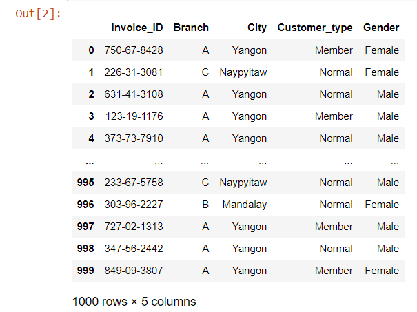
clean the dataset for visualization and statical analysis.
please check Data Preprocessing using python – Data Science (learntodatascience.com) for data preprocessing.
Data Visualization part:
use to plot graph
use plot graph
def univariate(df,col,vartype,hue =None):

    sns.set(style="darkgrid")

    if vartype == 0:
        fig, ax=plt.subplots(nrows =1,ncols=3,figsize=(20,5))
        ax[0].set_title("Distribution Plot")
        sns.distplot(df[col],ax=ax[0])
        ax[1].set_title("Violin Plot")
        sns.violinplot(data =df, x=col,ax=ax[1], inner="quartile")
        ax[2].set_title("Box Plot")
        sns.boxplot(data =df, x=col,ax=ax[2],orient='v')

    if vartype == 1:
        temp = pd.Series(data = hue)
        fig, ax = plt.subplots()
        width = len(df[col].unique()) + 6 + 4*len(temp.unique())
        fig.set_size_inches(width , 6)
        ax = sns.countplot(data = df, x= col, order=df[col].value_counts().index,hue = hue)
        if len(temp.unique()) > 0:
            for p in ax.patches:
                ax.annotate('{:1.1f}%'.format((p.get_height()*100)/float(len(loan_df))), (p.get_x()+0.05, p.get_height()+10))
        else:
            for p in ax.patches:
                ax.annotate(p.get_height(), (p.get_x()+0.25, p.get_height()+5))
        del temp
    else:
        exit

    plt.show()
calculate the branch wise average sales, total sales and total number of sales
df[['Branch', 'Total']]\
.groupby('Branch').agg(['mean','sum','count'])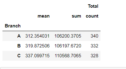
Find the total amount by date.
dates = df[['Date','Total']].groupby('Date').sum()
dates 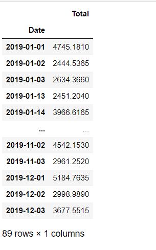
Resampling the sales total by one month and using mean to visualize the sales trend.
dates.resample('1M').mean().plot(figsize=(9,4))
Calculate the gender wise sales count
tq_genderwise = df[['Gender','Quantity']]\
.groupby(['Gender'], as_index=False).sum()
tq_genderwise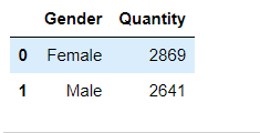
plt.figure(1, figsize=(20,10))
the_grid = GridSpec(2, 2)

plt.subplot(the_grid[0, 1], aspect=1, title='Total sales by  Gender')
type_show_ids = plt.pie(tq_genderwise.Quantity, labels=tq_genderwise.Gender, autopct='%1.1f%%', shadow=True, colors=colors)
plt.show()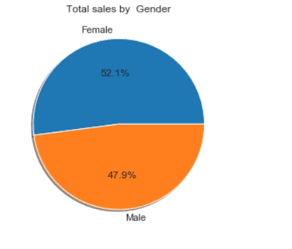
Customer type wise sales calculation
customer_wise = df[['Customer_type', 'Total']]\
.groupby('Customer_type').agg(['count','sum',])
customer_wise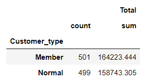
customer_wise = new_df[['Customer_type','Quantity']]\
.groupby(['Customer_type'], as_index=False).sum()
plt.figure(1, figsize=(20,10))
the_grid = GridSpec(2, 2)

plt.subplot(the_grid[0, 1], aspect=1, title='Total sales by  Customer Type')
type_show_ids = plt.pie(customer_wise.Quantity, labels=customer_wise.Customer_type, autopct='%1.1f%%', shadow=True, colors=colors)
plt.show()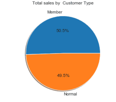
Payment wise sales calculation
 payment_wise_sales = new_df[['Payment','Quantity']]\
.groupby(['Payment'], as_index=False).sum()
payment_wise_sales
 payment_wise = new_df[['Payment','Quantity']]\
.groupby(['Payment'], as_index=False).sum()
plt.figure(1, figsize=(20,10))
the_grid = GridSpec(2, 2)

plt.subplot(the_grid[0, 1], aspect=1, title='Customer Payment Type')
type_show_ids = plt.pie(payment_wise.Quantity, labels=payment_wise.Payment, autopct='%1.1f%%', shadow=True, colors=colors)
plt.show()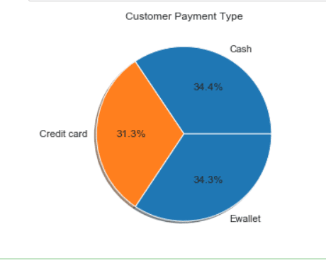
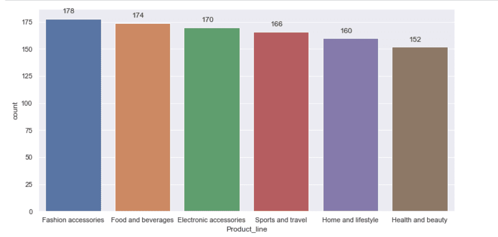
Product wise sales summary
 sales_product_wise = new_df[['Product_line', 'Total']]\
.groupby('Product_line').agg(['count','sum',])
sales_product_wise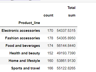
univariate(df=new_df,col='Product_line',vartype=1)